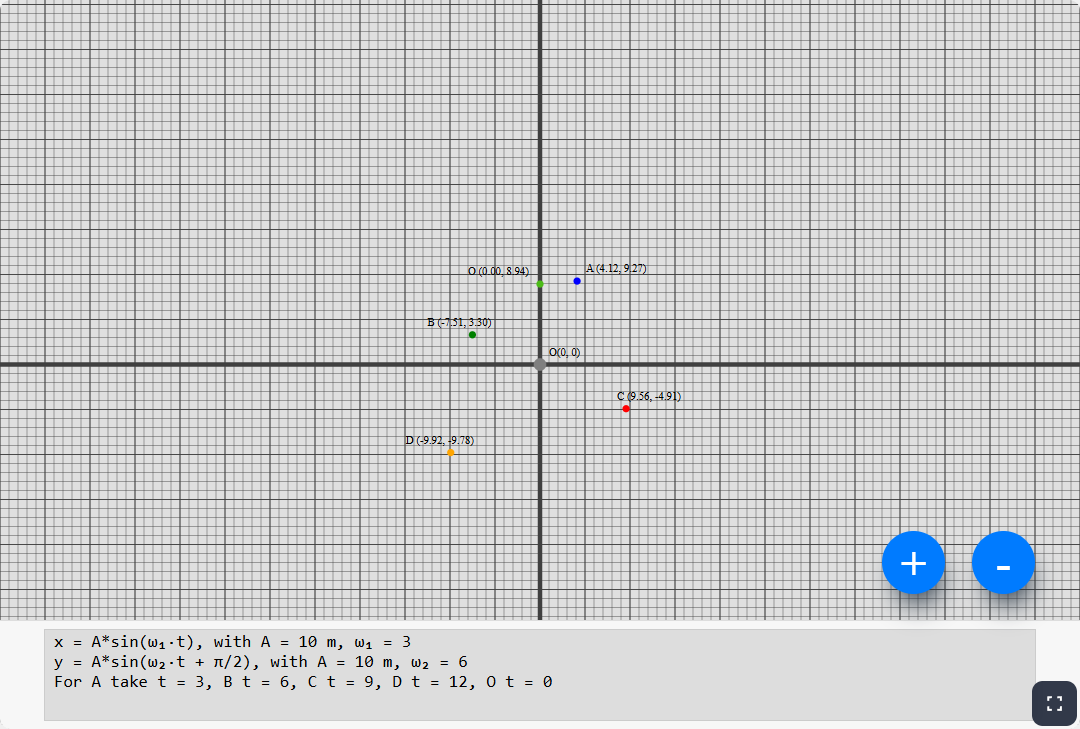
Lissajous figures
Two oscillations combine to trace a graph called a Lissajous curve (often pronounced “Liss-uh-joo”). One oscillation drives the x coordinate and the other drives y. The curve shows how both motions evolve together in time.
When the frequency ratio is rational (expressible as a ratio of integers a/b), the curve closes and retraces the same loop. Different ratios give different shapes.
Lissajous figures are plane curves that describe motion obtained by combining two perpendicular sinusoidal oscillations with different frequencies and phases.
They are named after Jules Antoine Lissajous, who studied them in the 19th century.
They are plotted using parametric equations and appear on an oscilloscope when two electrical signals drive perpendicular axes.
They are commonly used to study frequency and phase relationships between two signals.
Examples of Lissajous figures
The shape depends on the frequency ratio and the phase difference between the two oscillations.
Lissajous plot from parametric equations
This plot shows how x and y evolve from the parametric equations. Notice how different frequency ratios and phase shifts change the shape of the figure.