Mechanics — oscillatory motion and collisions

Mechanics studies how bodies move and the forces that cause motion. Here we focus on oscillatory motion and collisions — the foundation for understanding many more complex phenomena.

Oscillatory motion repeats periodically in time and appears in almost every physical system, from pendulums to atomic vibrations. Restoring forces tend to bring the system back toward equilibrium.

Collisions are processes in which two or more bodies interact through contact forces for a short time, exchanging momentum and kinetic energy according to conservation laws.

Harmonic oscillation along the x-axis

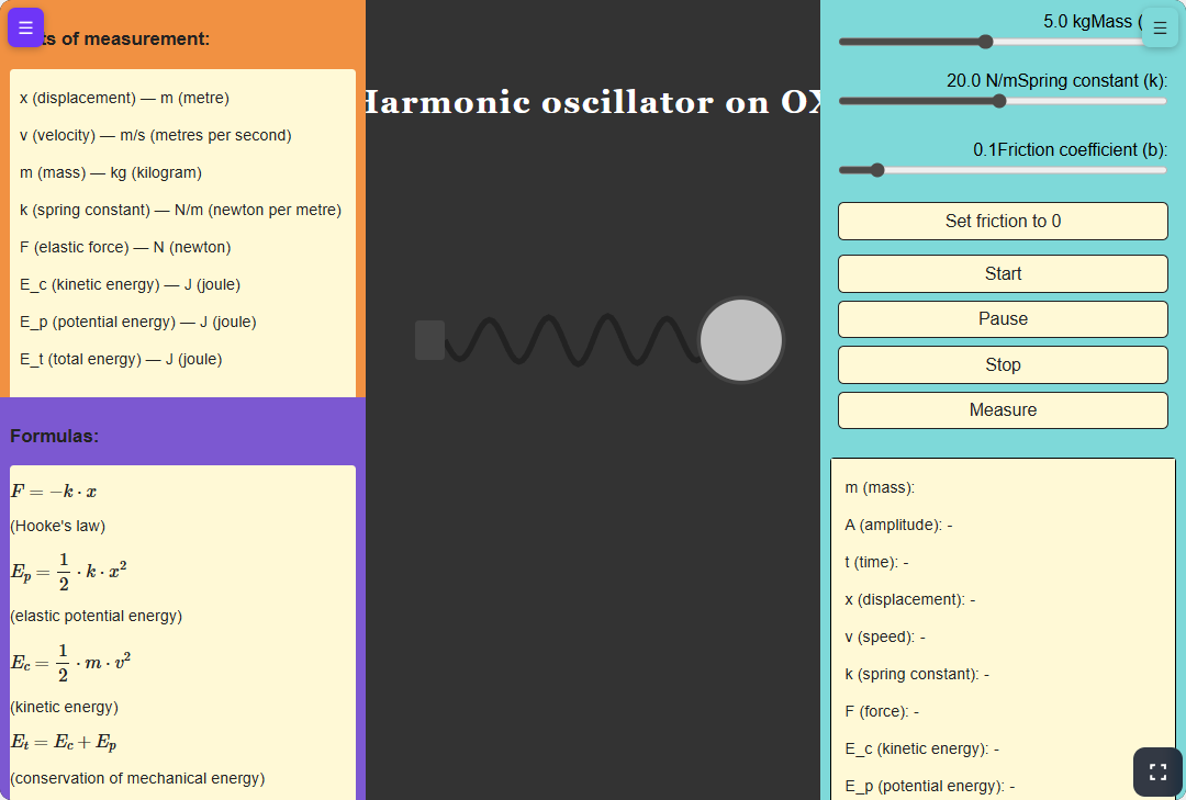
Motion along OX describes horizontal oscillation of a body under a restoring force proportional to displacement. It is central to understanding oscillator response in time.

When the body is displaced from equilibrium on OX, the restoring force F = −kx (Hooke's law) pulls it back. This yields simple harmonic motion with explicit equations for position, velocity and acceleration.

Harmonic oscillation along OX — simulation screenshot

Equations for harmonic oscillation along OX:

1. Equation of motion:

x (t) = A \sin (ω t + ϕ)

2. Velocity:

v (t) = ω A \cos (ω t + ϕ)

3. Acceleration:

a (t) = - ω^{2} A \sin (ω t + ϕ)

4. Angular frequency:

ω = \sqrt{\frac{k}{m}}

5. Oscillation period:

T = 2 π \sqrt{\frac{m}{k}}

where: A is the amplitude, ω is the angular frequency, φ is the initial phase, k is the spring constant, m the mass of the body and t time.

Harmonic oscillation along the vertical axis (OY)

The vertical harmonic oscillator models a mass on a spring oscillating vertically — gravity and elastic force combine.

Equilibrium is no longer at x = 0; it shifts to where the spring force balances weight, depending on mass and spring constant.

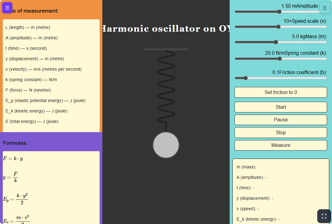
Vertical harmonic oscillation — simulation screenshot

Equations for harmonic oscillation along OY:

1. Equilibrium position:

y_{0} = \frac{m g}{k}

2. Equation of motion:

y (t) = y_{0} + A \sin (ω t + ϕ)

3. Velocity:

v (t) = ω A \cos (ω t + ϕ)

4. Total energy:

E = \frac{1}{2} m v^{2} + \frac{1}{2} k y^{2} + m g y

5. Natural frequency:

f = \frac{1}{2 π} \sqrt{\frac{k}{m}}

where: y₀ is the equilibrium position, A the amplitude, ω the angular frequency, φ the initial phase, k the spring constant, m the mass and g gravitational acceleration.

Collisions

Collisions are central in mechanics: two or more bodies interact through contact forces for a short time. They are essential for understanding momentum and energy conservation.

During a collision internal interaction forces dominate external ones, so conservation principles apply. Main types: elastic (kinetic energy conserved) and inelastic (part of kinetic energy converted to other forms).

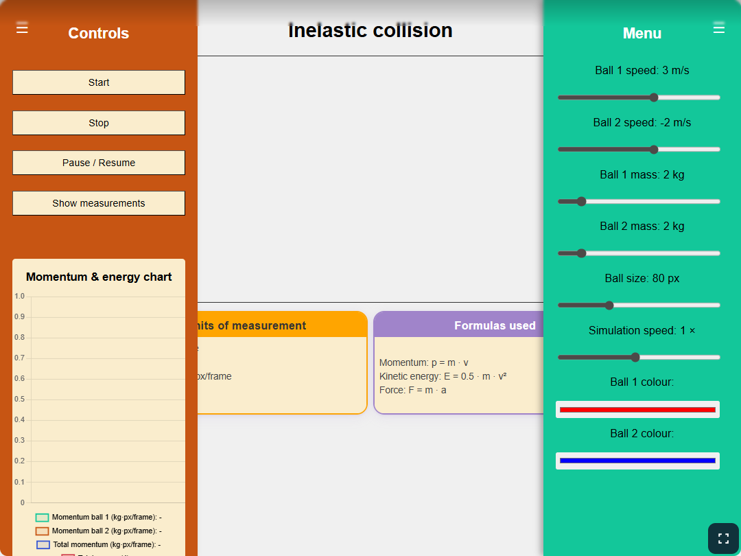
Collision formulas:

1. Conservation of momentum:

m_{1} v_{1 i} + m_{2} v_{2 i} = m_{1} v_{1 f} + m_{2} v_{2 f}

2. Coefficient of restitution:

e = \frac{v_{2 f} - v_{1 f}}{v_{1 i} - v_{2 i}}

3. Final speeds (elastic collision)::

v_{1 f} = \frac{(m_{1} - m_{2}) v_{1 i} + 2 m_{2} v_{2 i}}{m_{1} + m_{2}}

4. Final speed 2 (elastic):

v_{2 f} = \frac{(m_{2} - m_{1}) v_{2 i} + 2 m_{1} v_{1 i}}{m_{1} + m_{2}}

5. Kinetic energy in elastic collisions:

\frac{1}{2} m_{1} v_{1 i}^{2} + \frac{1}{2} m_{2} v_{2 i}^{2} = \frac{1}{2} m_{1} v_{1 f}^{2} + \frac{1}{2} m_{2} v_{2 f}^{2}

6. Momentum / impulse:

\vec{p} = m \vec{v}

where: m₁, m₂ are masses, v₁ᵢ, v₂ᵢ initial speeds, v₁f, v₂f final speeds, e is the coefficient of restitution (e = 1 perfectly elastic, e = 0 perfectly inelastic).

Inclined plane

The inclined plane is a classic setting for force analysis: weight splits into components that drive motion along the slope.

It links force, acceleration and potential energy and is the basis for many mechanics and engineering problems.

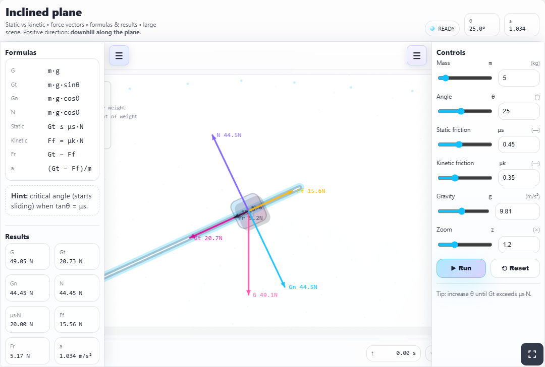
Formulas for the inclined plane:

1. Parallel component of weight:

F_{| |} = m g \sin (α)

2. Perpendicular component of weight:

F_{⊥} = m g \cos (α)

3. Friction force:

F_{f} = μ N = μ m g \cos (α)

4. Acceleration on the incline:

a = g (\sin (α) - μ \cos (α))

5. Speed at the bottom:

v = \sqrt{2 g h (1 - μ \cot (α))}

6. Time to descend:

t = \sqrt{\frac{2 h}{g (\sin (α) - μ \cos (α))}}

where: m is mass, g gravitational acceleration, α slope angle, μ friction coefficient, h vertical height of the plane, N the normal force.

Projectile motion

Projectile motion describes a body launched with initial speed in a uniform gravitational field (air resistance usually neglected). It combines uniform horizontal motion with uniformly accelerated vertical motion.

The path is parabolic for given launch speed and angle. The simulator lets you vary angle, speed and launch height to see range, maximum height and time of flight.

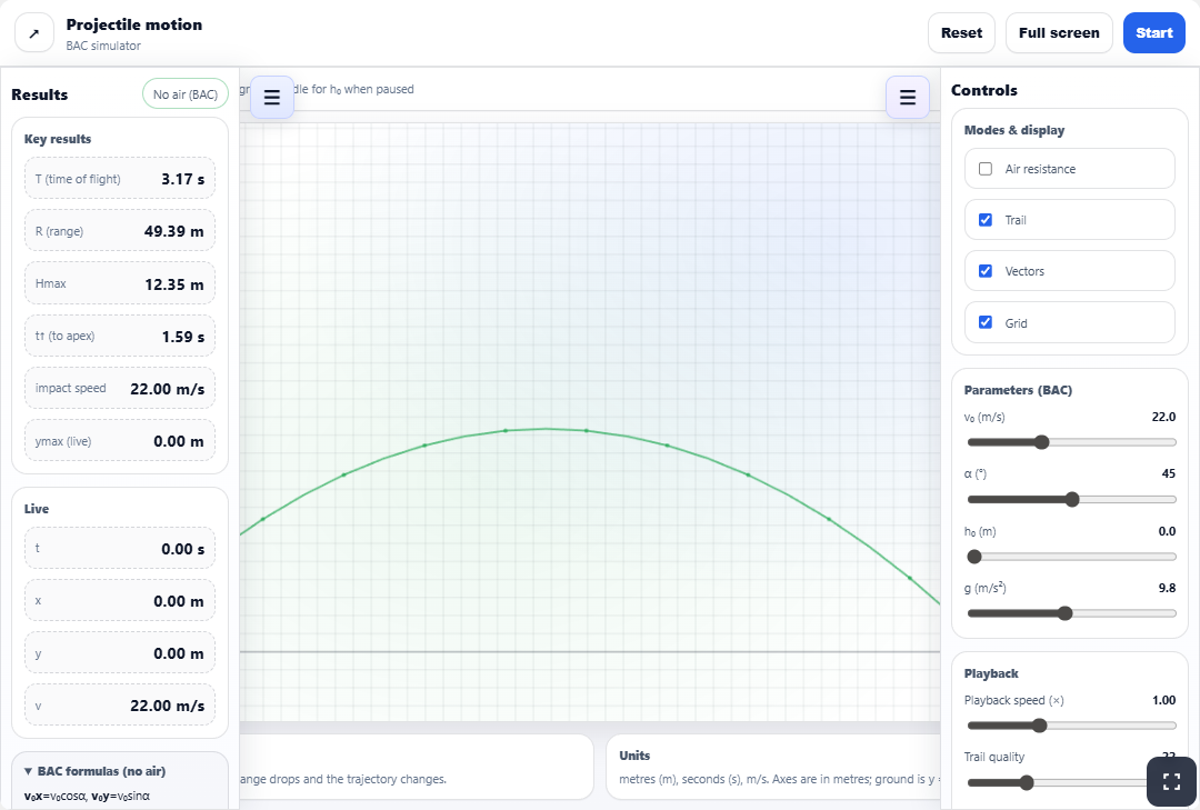
Projectile formulas (no air resistance):

1. Resolving the initial velocity:

v_{0 x} = v_{0} \cos α, v_{0 y} = v_{0} \sin α

2. Equations of motion::

x (t) = v_{0 x} t

3. Motion along OY:

y (t) = y_{0} + v_{0 y} t - \frac{1}{2} g t^{2}

4. Time of flight:

T = \frac{2 v_{0} \sin α}{g}

5. Horizontal range:

R = \frac{v_{0}^{2} \sin (2 α)}{g}

where: v₀ is initial speed, α launch angle above the horizontal, g gravitational acceleration, y₀ initial height, T time of flight, R horizontal range.

Elastic chains

An elastic chain consists of masses connected by Hookean springs. It models wave propagation in a discrete medium and collective motion of coupled oscillators.

You can watch how a disturbance propagates along the chain, reflections at ends, and how energy is shared among masses — linking discrete models to continuous waves.

Basic formulas for an elastic chain:

1. Spring force (Hooke's law):

F = - k Δ x

2. Equation of motion for a mass in the chain:

m \frac{d^{2} x_{i}}{d t^{2}} = k (x_{i + 1} - x_{i}) - k (x_{i} - x_{i - 1})

where: m is each mass, k the spring constant, and xᵢ the displacement of mass i from equilibrium. Neighbour differences produce forces that carry the disturbance along the chain.

Air resistance (aerodynamic drag)

When a body moves through a fluid (air, water, …), the fluid exerts a drag force opposing motion. In the usual turbulent regime it grows roughly with the square of speed.

Shape, cross-sectional area and fluid density set how large the drag is — e.g. a flat sheet falls differently from the same paper crumpled into a ball. When drag balances weight, the body reaches terminal speed and stops accelerating.

Drag matters in aerospace, ballistics, sports and vehicle design. The Reynolds number tells whether flow is laminar or turbulent and strongly affects drag.

Air-resistance formulas:

1. Drag force:

F_{d} = \frac{1}{2} C_{d} ρ A v^{2}

2. Equation of motion with drag:

m a = m g - \frac{1}{2} C_{d} ρ A v^{2}

3. Terminal speed:

v_{t} = \sqrt{\frac{2 m g}{C_{d} ρ A}}

4. Speed vs time:

v (t) = v_{t} \tanh (\frac{g t}{v_{t}})

5. Position vs time:

y (t) = \frac{v_{t}^{2}}{g} \ln (\cosh (\frac{g t}{v_{t}}))

6. Reynolds number:

Re = \frac{ρ v L}{μ}

where: C_d is the drag coefficient (shape-dependent), ρ fluid density (≈ 1.225 kg/m³ for air at sea level), A cross-sectional area, v speed, m mass, g gravity, v_t terminal speed, Re Reynolds number, L a characteristic length and μ dynamic viscosity.