Nuclear physics

This page brings together materials on induced fission in U-235, an educational D–T fusion model, heavy water and deuterium separation (isotope exchange, distillation), and—at the end—two uranium-isotope simulations (four key isotopes and the chart of all 26). The simulators are not substitutes for nuclear engineering curricula or safety analysis; they support intuition and high-school curricula.

Below: chain fission (U-235), D–T fusion, D₂O vs H₂O, isotope exchange and fractional distillation; lastly, uranium isotopes (four essentials plus the chart of 26).

Simulator: Nuclear chain fission (U-235)

A thermal neutron can be captured by a U-235 nucleus (²³⁵₉₂U); the compound nucleus breaks into fission fragments, fresh neutrons (on average 2–3 per fission for U-235) and gamma rays. When each generation yields more than one neutron usable for further fissions, the effective multiplication factor exceeds 1 and power rises—the idea behind controlled chain reactions with rods and moderator.

In the simulator each fission adds roughly 200 MeV to the cumulative energy (a pedagogical benchmark for energy per event). The displayed factor k is an empirical ratio between fission rates on successive time segments so you can discuss subcritical / critical / supercritical without claiming a complete reactor model.

U-235 chain fission simulator: neutrons, nuclei, k factor and cumulative energy

Formulas tied to the simulator model

1. Induced fission (schematic)

Neutron capture and fragments (nu = number of emitted neutrons; masses and Z depend on the fission channel):

_{92}^{235} U +_{0}^{1} n \to_{Z_{1}}^{A_{1}} X +_{Z_{2}}^{A_{2}} Y + ν_{0}^{1} n + γ

Conservation requires 235 + 1 = A₁ + A₂ + nu and 92 = Z₁ + Z₂.

2. Cumulative energy (simulation baseline)

Let N count fissions and averaged E mean energy released per fission (200 MeV in the app):

E_{tot} \approx N ⟨ E ⟩

3. Mass defect and reaction energy (Q)

Q = (m_{U} + m_{n} - m_{frag 1} - m_{frag 2} - ν m_{n}) c^{2}

Typical order of magnitude: Q of tens of MeV per emitted nucleon; total per fission on the hundreds of MeV—that is why the teaching model rounds to ~200 MeV.

4. The k factor (simulator viewpoint)

In a generation picture the multiplication factor is written as the ratio of useful neutrons between successive generations. The app estimates an empirical k from the evolution of the fission rate, not microscopic cross sections:

k = \frac{N_{i + 1}}{N_{i}} (model simplificat)

k < 1 subcritical; k ~= 1 critical (on average stable); k > 1 supercritical—power rises unless cooling/absorption intervene (SCRAM rods in simulation).

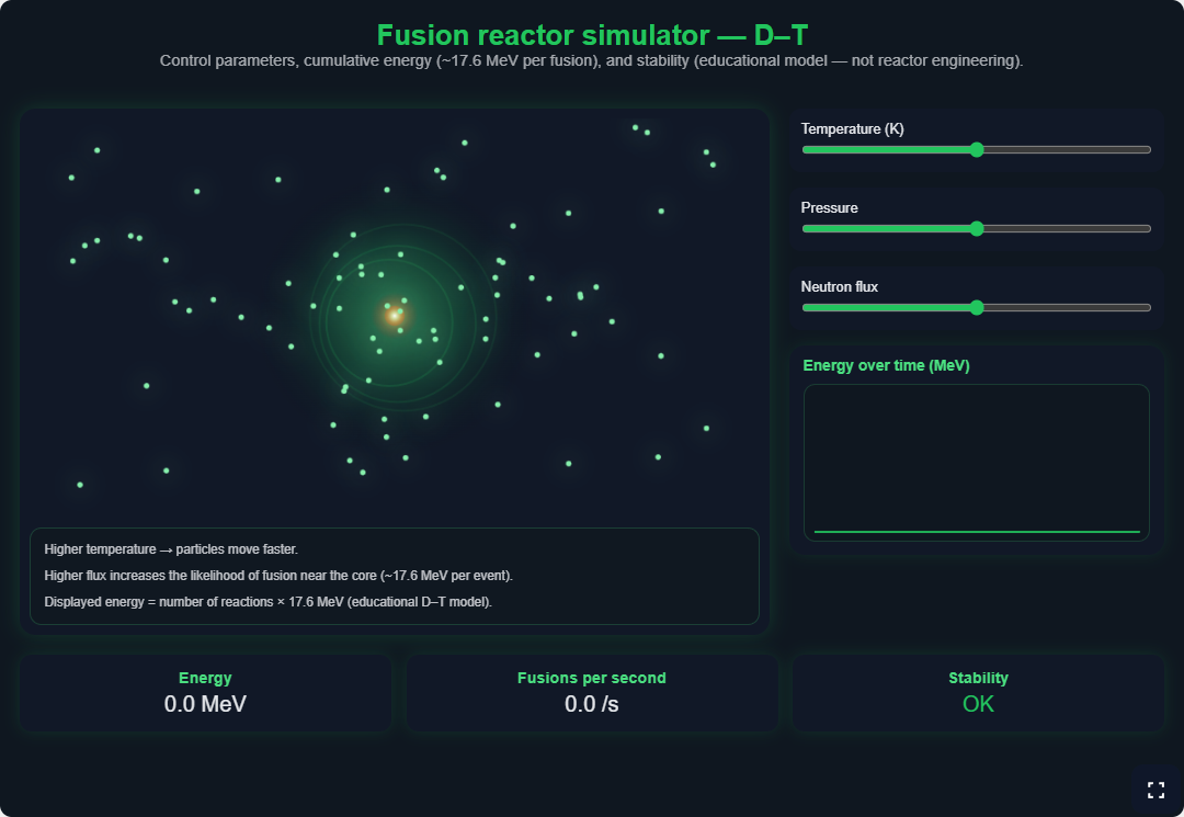
Simulator: D–T fusion reactor

Each fusion event near the nucleus in the simulator adds 17.6 MeV—the standard textbook value for a deuterium plus tritium reaction. Controls (temperature, pressure, neutron flux) tune particle speeds, overlap probability near the nucleus and stability; beyond a critical threshold the demonstration switches into a purely illustrative meltdown scenario.

Parameters in the UI: temperature (0–1000 K), pressure (0–100 relative scale), neutron flux (0–10). The fusion zone widens mildly with cumulative energy; meltdown triggers when flux exceeds ~8.5 while temperature exceeds ~850 K simultaneously.

Educational D–T fusion reactor simulator: core, particles, controls and energy plot

Formulas tied to the simulator model

1. D + T fusion reaction

Sketch (particles emitted and indicative energy released):

_{1}^{2} H +_{1}^{3} H \to_{2}^{4} He +_{0}^{1} n + 17, 6 MeV

Tritium is unstable (beta minus), so in practice tritium must be bred or regenerated in a reaction chain—the simulator highlights only the ~17.6 MeV benchmark per event.

2. Displayed cumulative energy

Let N count fusion events in the simulation:

E_{tot} = N \cdot 17, 6 MeV

The energy-vs-time graph tracks sampled E_tot inside the animation loop; Fusions/s estimates events inside the latest second via timestamps.

3. Mass defect and Q

Released energy links the masses of reactants and products:

Q = (m_{D} + m_{T} - m_{He} - m_{n}) c^{2}

Q ~ 17.6 MeV for D–T is the simulator benchmark per event; in a real reactor energy is shared among particles and structure—confinement and materials are not modelled.

4. Stability and critical thresholds (simulation only)

The app shows qualitative states such as OK / unstable before meltdown; triggering is effectively large flux AND large temperature simultaneously. There is no single universal physics formula—just a pedagogical threshold for discussing power feedback and cooling.

Brief history and Romanian context

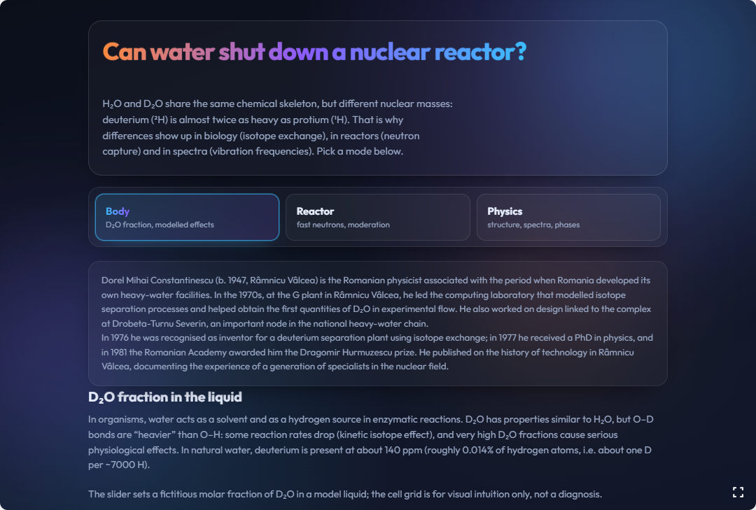
In Romania debates about heavy water tie into nuclear infrastructure and the era when national facilities separated deuterium isotopes. Physicist Dorel Mihai Constantinescu is associated with process modelling relevant to manufacturing D₂O.

In the 1970s at Plant G in Râmnicu Vâlcea he worked on computing and simulation of processes aimed at obtaining heavy water, bridging from design concepts to tangible experimental milestones.

For students this link helps show that heavy water is not only formulae—it belongs to Romanian nuclear-engineering history, to the moderator role in reactors, and to how research, engineering and simulation worked together.

What the heavy-water simulator compares (D₂O vs H₂O)

Code-wise the Body section uses an educational slider for a fictitious molar fraction of D₂O with a coloured status ladder (explicitly labelled as educational only). Physics compares indicative properties (boiling point, density, frequency), while Reactor sketches schematic neutron-capture contrasts for D₂O versus H₂O.

Heavy-water moderator simulator screenshot

Formulas and relations used for D₂O / H₂O comparison

1. D₂O mole percentage (Body mode)

For a mixture modelled by the simulator, the D₂O percentage is:

x_{D_{2} O} (%) = 100 \cdot \frac{n_{D_{2} O}}{n_{D_{2} O} + n_{H_{2} O}}

The fraction is illustrative for intuition; not a clinical instrument nor a direct depiction of physiological concentration.

2. Ratio of vibrational frequencies (Physics mode)

Harmonic oscillator style: frequency scales inversely with the square root of reduced mass:

f \propto \frac{1}{\sqrt{μ}}, \frac{f_{D_{2} O}}{f_{H_{2} O}} \approx \sqrt{\frac{μ_{H_{2} O}}{μ_{D_{2} O}}}

The simulator reduced-mass-ratio slider embodies heavier D₂O giving lower characteristic frequencies.

3. Differences at phase transitions

Difference between indicative boiling and freezing temperatures:

Δ T_{b} = T_{b} (D_{2} O) - T_{b} (H_{2} O), Δ T_{f} = T_{f} (D_{2} O) - T_{f} (H_{2} O)

Orientative simulator values include T_b(H₂O) ~ 100.0 °C versus T_b(D₂O) ~ 101.4 °C, and freezing near 0 °C versus ~ 3.8 °C.

Isotope-exchange plant (H₂S–H₂O)

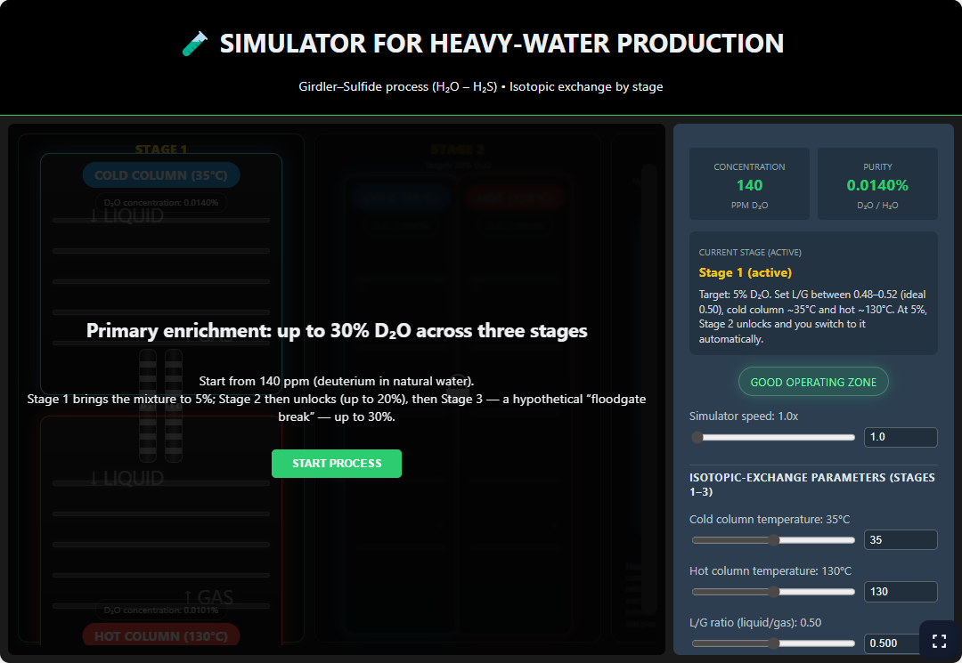
This simulator sketches how isotope-exchange enriches deuterium in water. Beyond the textbook formula alone you witness stage-wise effects, mass transfer and overall efficiency tendencies.

The model is educational—meant for main trends of isotopic separation rather than sizing a real industrial unit.

In Romanian technological history Constantinescu detailed why separating heavy water is hard: chemistry of H₂O and D₂O is nearly alike, useful distinctions are mostly physical, while raising enrichment from roughly 140 ppm natural abundance to reactor-grade ~99.8% demands sprawling plant and enormous energy expenditure.

Heavy-water isotope-exchange plant simulator screenshot

Interpretation formulas

1. Isotope separation factor

α = \frac{(x_{D} / (1 - x_{D}))_{f a z a A}}{(x_{D} / (1 - x_{D}))_{f a z a B}}

The factor alpha shows how efficiently isotopes divide between phases at equilibrium. Larger alpha means more enrichment per ideal stage.

2. Mass balance for deuterium

F x_{F} = P x_{P} + W x_{W}

Relates feed flow F at concentration x_F to product P and waste W streams.

3. Progressive enrichment across stages (simplified pedagogy)

x_{D}^{(n)} \approx x_{D}^{(0)} α^{n}

(aprox. didactică)

Higher useful stage count n boosts deuterium concentration when each stage contributes net separation.

4. Two-step technology sketch

Industrial descriptions for Plant G emphasise primary enrichment (large flow, modest concentration, dominates energy demand) versus finishing flows (tiny throughput pushing up to ~99.8% D₂O).

The canonical scheme chains H₂O–H₂S isotope-exchange in thermal columns (cold + hot towers) with vacuum distillation / rectification for the final polishing step—the simulator conveys cascade logic and optimisation of liquid-to-gas ratio.

Fractional distillation: from ~20% to reactor-grade heavy water

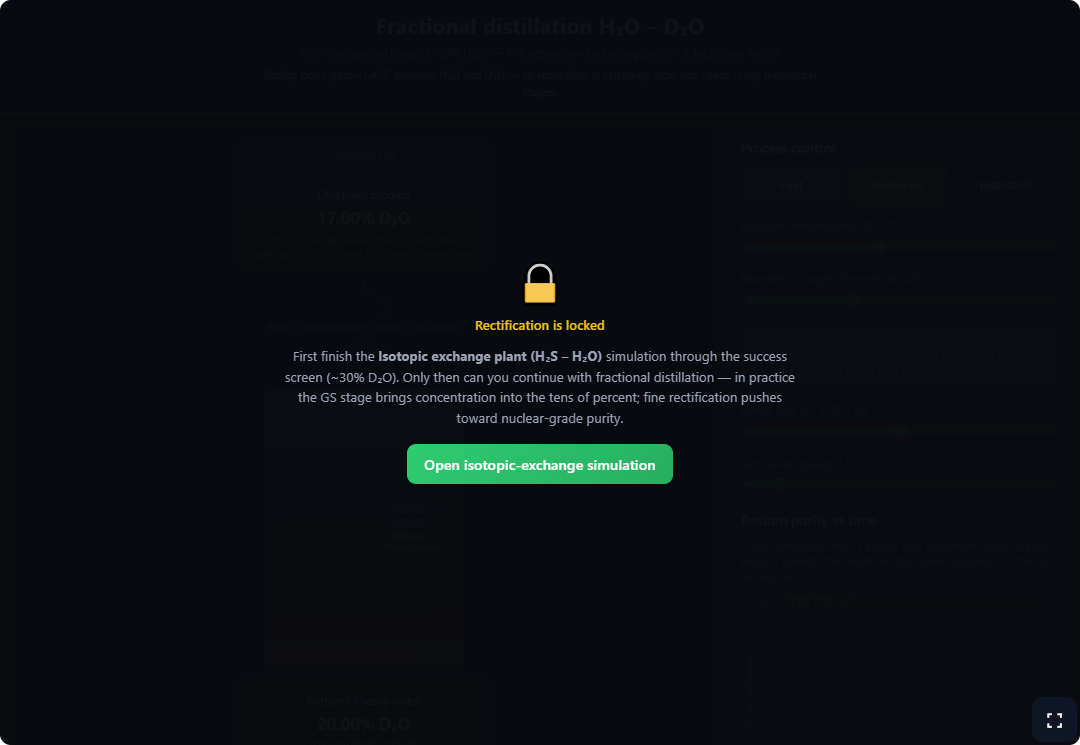
After isotope-exchange drives concentrations toward tens-of-percent regimes, polishing relies on the small boiling gap between H₂O and D₂O (~1.4 °C): a rectification tower with many stages, vigorous reflux and a bottom reboiler concentrates D₂O at the column bottom while vapour leaning toward H₂O rises toward the condenser.

The schematic tracks purity versus time alongside reflux influence and theoretical stages—emphasising why the last fractions toward ~99.8% are the costliest; the fractional-distillation simulator stays locked until the exchange simulation finishes (saved locally).

$H₂O–D₂O fractional distillation simulator: column, reflux and purity plot$

Helpful formulas for rectification

1. Relative volatility (light/heavy components)

Let L denote the more volatile fraction (H₂O) and H the less volatile (D₂O); at equilibrium:

α_{L / H} = \frac{(y_{L} / x_{L})}{(y_{H} / x_{H})}

For H₂O/D₂O, relative volatility is close to simulator default ~1.06, so each stage barely separates—that many stages plus high reflux.

2. Vapour–liquid equilibrium (light-component mole fractions)

With liquid and vapour mole fractions x, y for H₂O and constant pedagogical alpha:

y = \frac{α x}{1 + (α - 1) x}

Liquid D₂O mole fraction equals 1 − x; at the column bottom rectification lowers x raising D₂O fraction.

3. Internal reflux

R = \frac{L}{D}

L is reflux molar flow returning downward, D the overhead draw-off. Larger R improves separation but trims light-product throughput and lengthens timelines toward ultrahigh bottoms purity.

4. Minimum-stage count (Fenske, constant alpha)

Didactic estimate of stages needed under total reflux between distillate mole fraction x_D and bottoms fraction x_B of the light species:

N_{min} = \frac{\ln (\frac{x_{D} / (1 - x_{D})}{x_{B} / (1 - x_{B})})}{\ln α}

Real reflux ratios and efficiencies raise the actual stage count versus N_min; nonetheless alpha barely above 1 yields huge N for strong separation.

5. Tie to boiling-point gap

Distillation exploitation rests on differing boiling temperatures; Delta T_b = T_b(D₂O) - T_b(H₂O) (~1.4 °C) implies relative volatility exceedingly close to 1.

Simulator: Uranium isotopes (nucleus, alpha, fission, time)

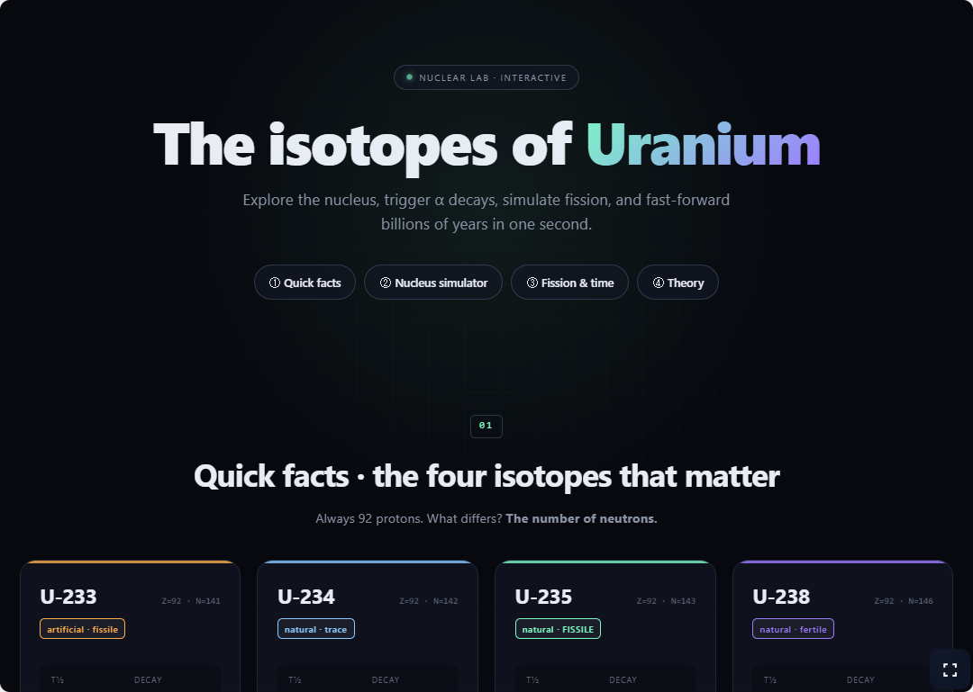
Uranium always has Z = 92 protons; isotopes differ by neutron count N hence mass number A = Z + N. The simulator spotlights four isotopes common in curricula (233…238 U): nucleus sketch, alpha decay (emission of ⁴₂He), a fission example on U‑235 plus a radioactive time machine using half-life-driven decay.

Uranium-isotope simulator: nucleus, N/Z ratio, alpha decay and time evolution

Model-linked formulas

1. Notation and neutron count

_{Z}^{A} X, A = Z + N

For uranium Z = 92; shorthand U-A denotes isotope.

2. Alpha decay sketch

_{Z}^{A} X \to_{Z - 2}^{A - 4} Y +_{2}^{4} He

In this simulation alpha emission reduces daughter Z by two nucleons lost by four from the parent.

3. Same exponential law as the time module

N (t) = N_{0} e^{- λ t}, λ = \frac{\ln 2}{T_{1 / 2}}

Interfaces may equivalently adopt half-power form.

Simulator: Chart of uranium’s 26 isotopes

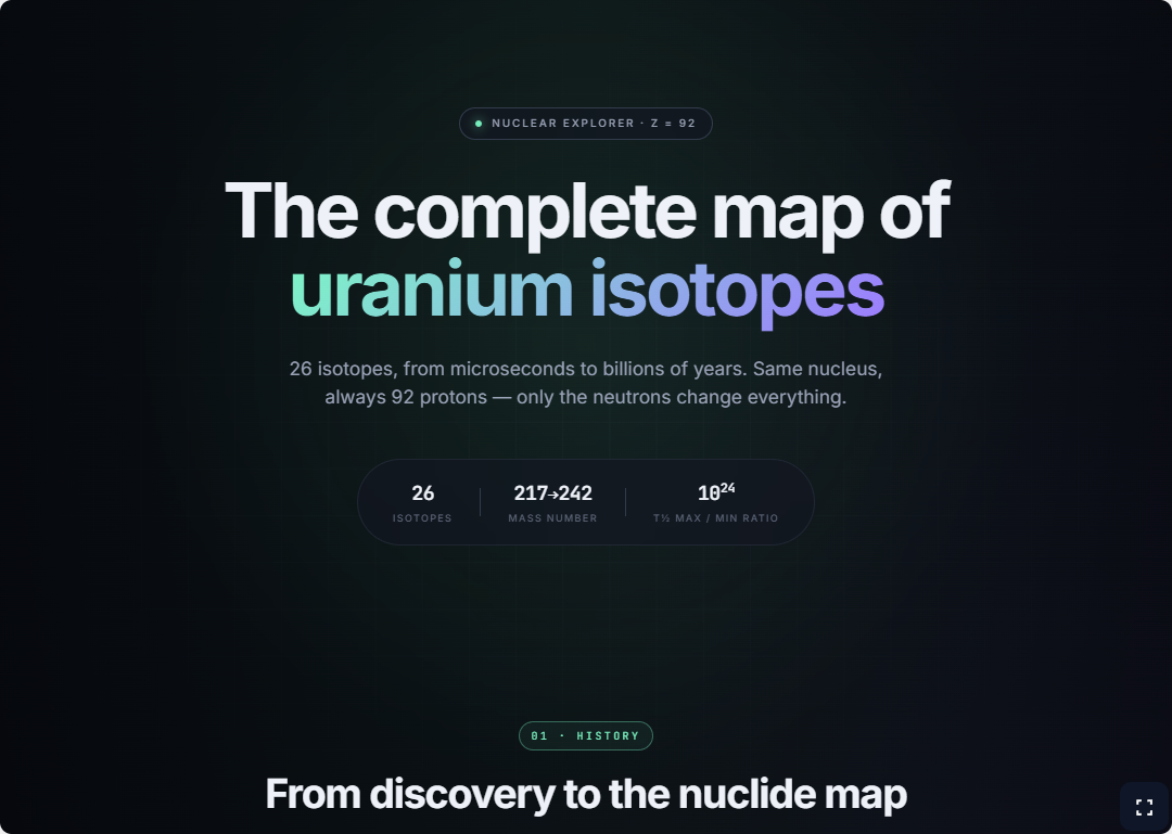
Experimentally 26 uranium isotopes are catalogued (mass numbers A spanning roughly 217–242). In nature prominent abundances boil down to U-234, U-235 and U-238; others arise in reactors or fleeting decay chains. The simulator colours dominant decay modes (alpha, beta minus, electron capture / beta plus), shows details upon selection, and overlays N(t) with lambda inferred from listed half-life.

Chart of uranium isotopes: cells along row Z = 92, legend of decay pathways

Useful formula (same law for each)

λ = \frac{\ln 2}{T_{1 / 2}}, N (t) = N_{0} e^{- λ t}

Cell brightness conveys relative stability; educational figures aggregate public summaries rather than authoritative nuclear evaluations.