Quantum physics

We introduce two core phenomena: amplitude superposition in the double-slit experiment (interference and probability) and penetration of a potential barrier (tunnelling). Below each simulation are commonly used formulas with short explanations.

Double-slit experiment

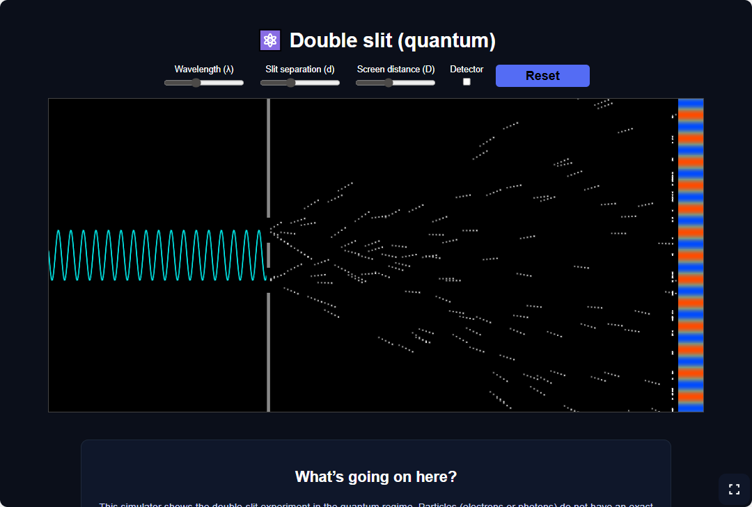
A beam passes through two parallel slits. In the quantum description the amplitude on the screen is the sum of contributions from each slit; measured intensity follows Born's rule and can show interference fringes. If you localize the particle on one path before the screen, the pattern changes — wave–particle complementarity.

Essential formulas (double slit)

Interference maxima

For two slits separated by distance d and wavelength λ, at angle θ to the symmetry axis the path difference is approximately d sin θ. Constructive interference (intensity maxima) when this difference is an integer number of wavelengths:

d \sin θ = m λ, m = 0, \pm 1, \pm 2, \dots

Fringe spacing (Young, small angle)

On a screen at distance L ≫ d from the slits, in the small-angle approximation sin θ ≈ y/L, the spacing between consecutive maxima of order m and m+1 on the screen is approximately:

Δ y \approx \frac{λ L}{d}

The closer the slits (small d) or the longer the wavelength, the farther apart the fringes on the screen.

Born rule (probability)

The probability of detecting the particle in a small region of space is proportional to the squared modulus of the wavefunction (the sum of amplitudes for all relevant paths):

P \propto | ψ |^{2}

That is why interference is seen: terms that add in ψ can produce maxima or minima of |ψ|², not merely a sum of independent intensities.

Quantum tunnelling

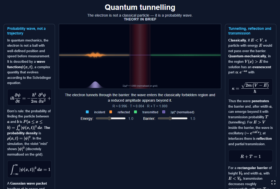
In regions where classically the kinetic energy would be negative (E < V(x)), the wavefunction does not vanish abruptly: inside the barrier an evanescent part appears that decays exponentially, so there is non-zero probability of finding the particle beyond the barrier — tunnelling. It occurs in tunnel diodes, scanning tunnelling microscopes (STM) and many nuclear and chemical models.

Essential formulas (tunnelling)

Time-independent Schrödinger equation (1D)

For a state with well-defined energy E, the time-independent form in one dimension is:

- \frac{ℏ^{2}}{2 m} \frac{d^{2} ψ}{d x^{2}} + V (x) ψ = E ψ

In each region where V is approximately constant, the solution is a combination of exponentials (oscillatory if E > V, growing/decaying if E < V).

Wavenumber in the allowed region and decay in the barrier

For a rectangular barrier of height V₀ and E < V₀, inside the barrier (where classically the particle would not pass) the evanescent solution involves the parameter κ:

κ = \frac{\sqrt{2 m (V_{0} - E)}}{ℏ}

The higher the barrier relative to E (i.e. the larger V₀ − E), the larger κ and the faster the wave decays inside the barrier.

Transmission through a thick barrier (idea)

For a sufficiently wide barrier of width a, the transmission coefficient (probability to pass) decreases very rapidly with width, often dominated by a factor of the form:

T \sim e^{- 2 κ a}

Exact numerical factors depend on the barrier shape (step, smooth, etc.), but the exponential dependence on κ a explains why tunnelling is sensitive to a few ångströms in STM or layer thickness in real devices.

Order of magnitude: energy and duration (Heisenberg)

A state that does not live forever (e.g. a metastable level) has an uncertainty in energy related to its characteristic lifetime Δt:

Δ E Δ t ≳ \frac{ℏ}{2}

Useful when estimating level widths or lifetimes in processes involving tunnelling from a confined state.

Bonding between atoms and molecular orbitals

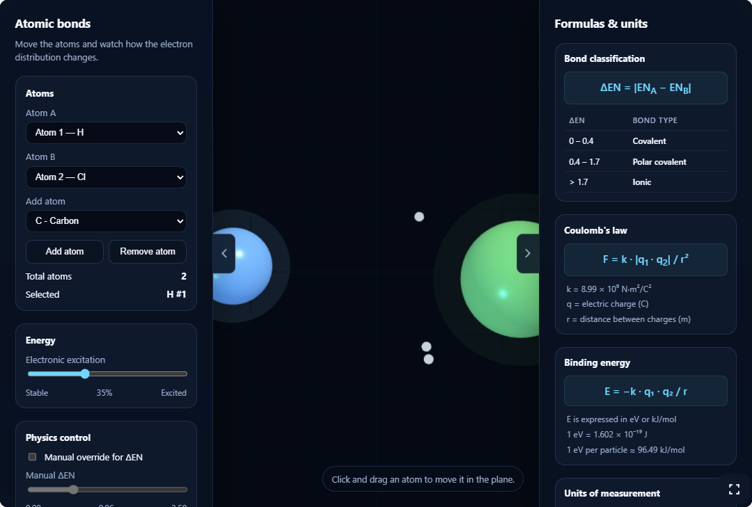
Beyond the isolated atom, quantum mechanics explains why atoms can bind into stable molecules: linear combinations of atomic orbitals lead to bonding and antibonding molecular orbitals. Increased probability density between nuclei corresponds to a lower total energy than separated atoms.

Essential formulas (atomic bonding)

Combining atomic orbitals (bonding / antibonding MOs)

In the very simplified picture of the H₂ molecule, two 1s orbitals can combine into a bonding (symmetric) and an antibonding (antisymmetric) orbital:

ψ_{leg} = c_{1} ψ_{A} + c_{2} ψ_{B}, ψ_{anti} = c_{1} ψ_{A} - c_{2} ψ_{B}

In the bonding orbital, the probability density |ψ_bond|² is larger between the nuclei, lowering the total energy compared to separated atoms.

Binding energy

Binding energy is defined as the difference between the energy of separated atoms and the energy of the molecule:

E_{leg} = E_{atomi separați} - E_{moleculă}

The larger E_bind, the stronger the bond and the more stable the molecule.

Binding force — harmonic oscillator approximation

Near the equilibrium separation r₀ between nuclei, the binding potential can be approximated by a harmonic oscillator:

F \approx - k (r - r_{0})

The effective constant k relates to bond “stiffness”; vibrational frequency depends on k and the reduced mass of the two atoms.

Probability density along the bond

The probability of finding electrons at point $\vec{r}$ is given by the probability density:

ρ (\vec{r}) = | ψ_{leg} (\vec{r}) |^{2}

High density between nuclei is the hallmark of a covalent bond; in the antibonding orbital this density is small or zero between nuclei.